An FBAR weighing a protein, a 77 GHz radar ranging a car, a lidar counting photons off a wall, and an interferometer measuring optical phase are four entirely different pieces of physics. They share exactly one thing.
σθ ≥ 1 / √J(θ) J = (∂s/∂θ)² / σ²n
Change the physics and you change the derivative. You do not change the law.
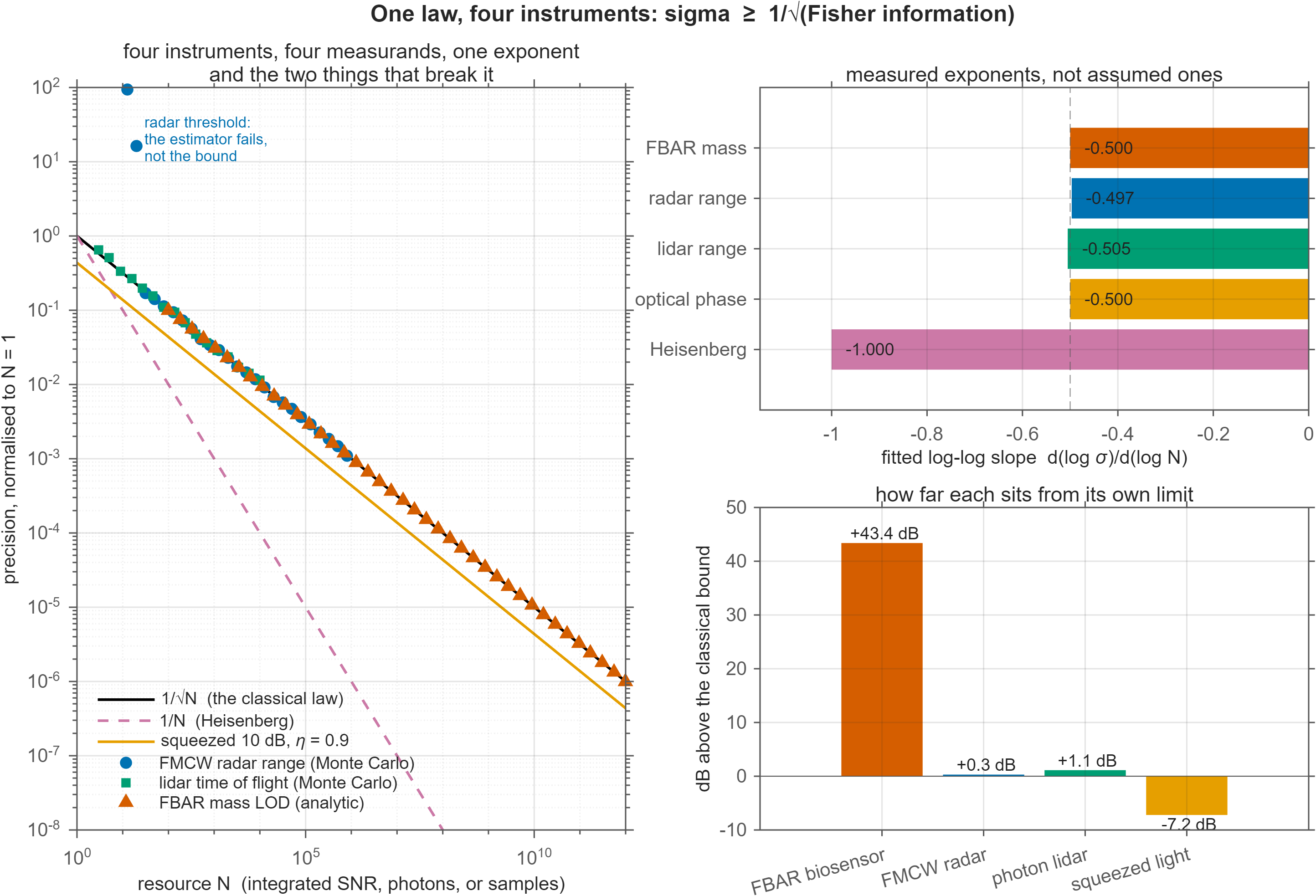
−0.500
fitted exponent, FBAR mass LOD
−0.497
fitted exponent, radar range
−0.505
fitted exponent, lidar range
26 / 26
physics assertions passing
−7.2 dB
the only thing below the line
The capstone
Four measurands, one exponent
Plotted against the resource each instrument spends — integrated SNR, photons, samples — all four fall on the same slope of −1/2. Not approximately. The radar and lidar points are Monte Carlo output from simulations in this repository, not curve fits, and their fitted exponents come out at −0.497 and −0.505.
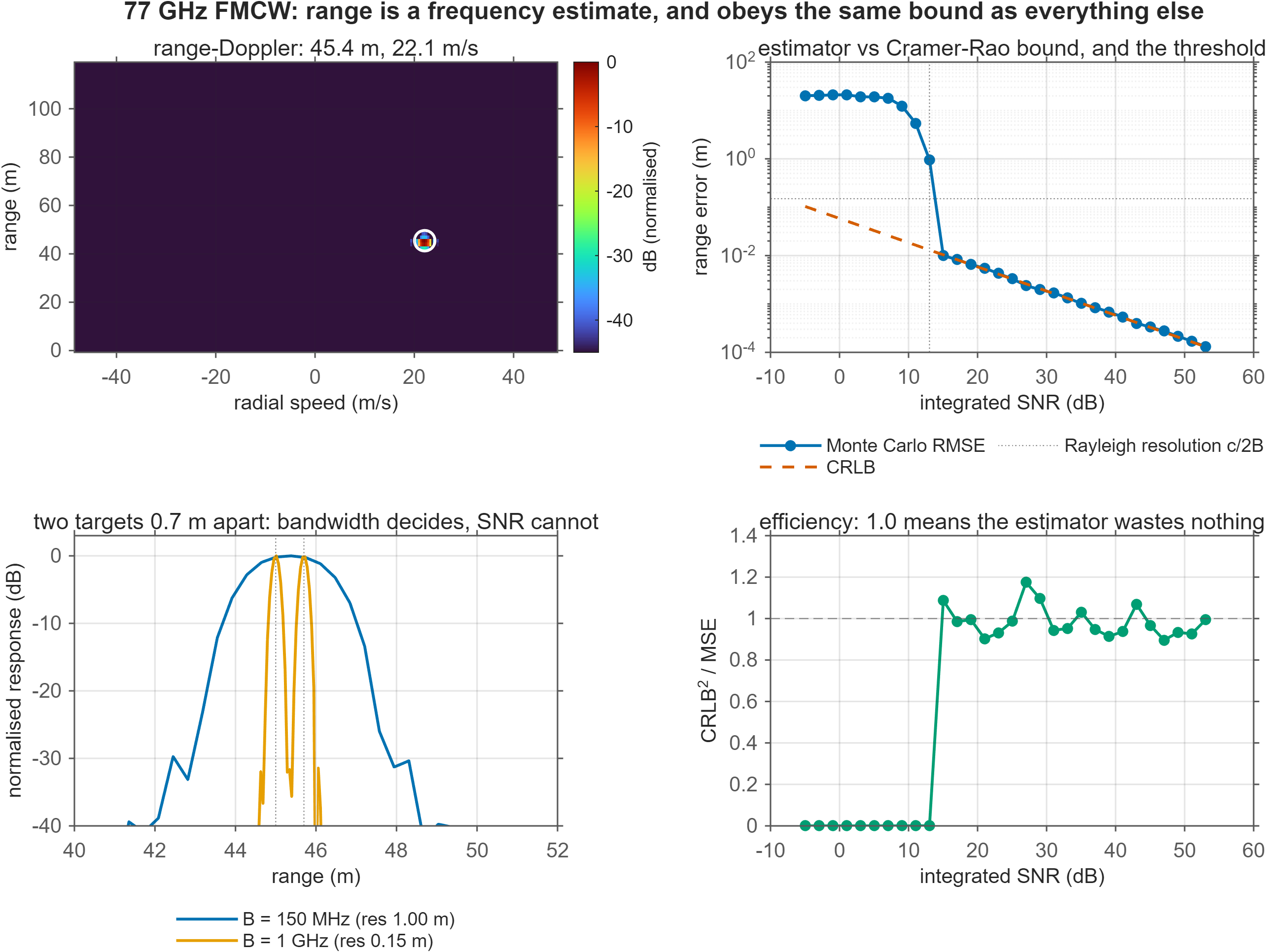
Two things break the pattern, and they are the interesting ones. The radar points leave the line below 13 dB integrated SNR — that is the estimator failing, not the bound failing, and it is the Rife–Boorstyn threshold. And the squeezed-light curve sits below the classical line while the Heisenberg curve has a different slope entirely. Those are the only two exits, and both require changing the probe's quantum statistics rather than the instrument's engineering.
The central result
Frequency buys you nothing
A film bulk acoustic resonator's Sauerbrey mass sensitivity grows as the square of its operating frequency, Sm = −2f₀²/Za. Every FBAR biosensor paper says so, usually in the abstract. A 2 GHz aluminium-nitride device shifts 2,229 Hz per ng/cm² against a 5 MHz quartz microbalance's 0.057 Hz — a factor of thirty-nine thousand.
But the frequency noise referred to the same measurement grows too. From the resonator's phase slope ∂φ/∂f = 2Q/f₀ and the phase-estimation bound σφ = 1/√(2·SNR), the f₀² cancels against the f₀:
LOD = k·Za / (4·Q·f₀·√(2·SNR)) ∝ Za / (Q·f)
And Q·f is pinned near a material constant by Akhiezer phonon damping — around 10¹³ Hz for AlN.
The consequence
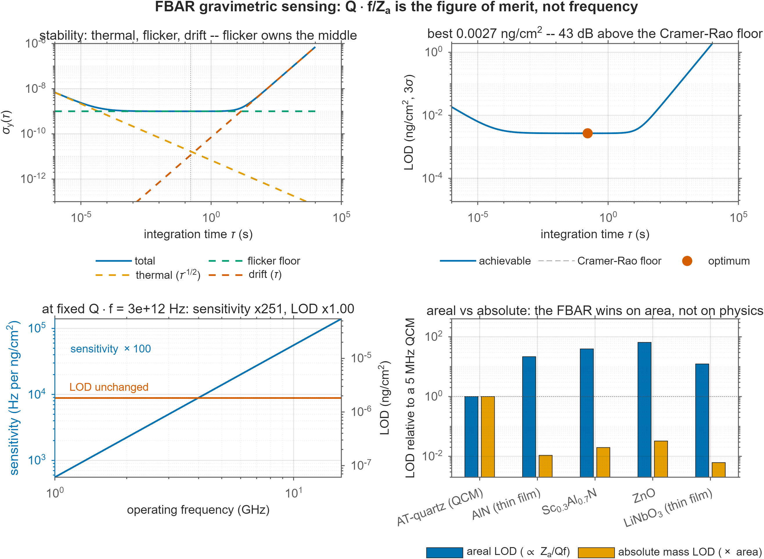
At fixed Q·f, raising the operating frequency does not lower the detection limit. From 1 GHz to 10 GHz the sensitivity rises by a factor of 251 and the LOD does not move at all.
The test suite asserts this to a relative tolerance of 1e−9. If the claim ever stops being true, the build goes red.
Bottom left is the whole argument in one panel. The levers that actually work are lower acoustic impedance, a better Q·f product, and more SNR — not more gigahertz. The material figure of merit is M = Q·f / Za, and the ranking it produces is not the one the field's marketing implies: a 5 MHz AT-cut quartz crystal has roughly twenty times the intrinsic areal figure of merit of a 2 GHz AlN FBAR. The FBAR wins on area — a 100 × 100 µm transducer against a 1 cm² disc is a factor of 5,000 in absolute mass — which more than repays the penalty. Bottom right separates the two honestly.
There is also a 43 dB gap between the Cramér–Rao floor and what the same device achieves once flicker noise and thermal drift are in the model. That gap is not a rounding error. It is where the entire engineering discipline lives.
Why Simulink is here and not decorative
The device, and the instrument
The MATLAB modules describe the device — an equivalent circuit, an impedance, a sensitivity, a bound. None of that is dynamic. The Simulink model describes the instrument around it, and it earns its place by producing a result the static analysis cannot.
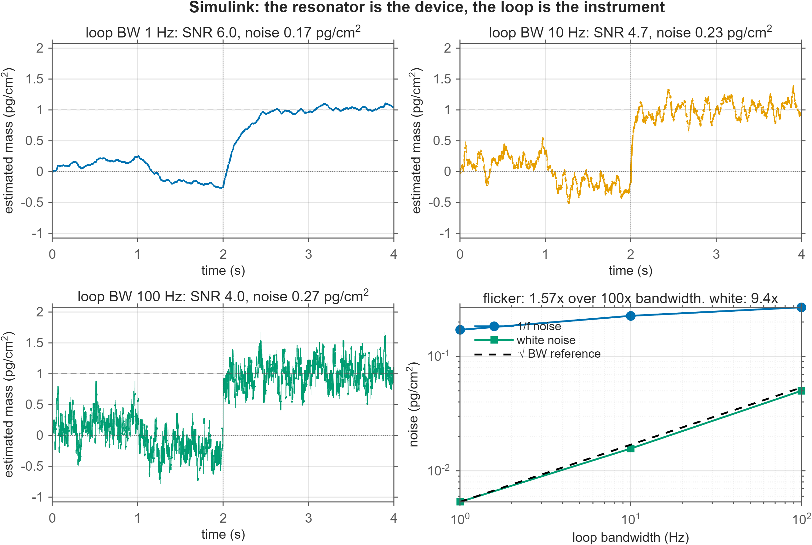
With white noise, narrowing the loop bandwidth buys you √BW — the familiar trade, reproduced to within 6% over two decades. With 1/f noise it buys almost nothing: a hundredfold reduction in bandwidth improves the noise by a factor of 1.57, at a hundredfold cost in response time. That is the flat bottom of the Allan bathtub expressed as a control system, and it is the reason resonant sensors are not improved by "just integrating for longer". Much harder to argue with when you can watch a 1 pg/cm² binding event arrive at SNR 6.
A note on the .slx
The model is built by script, not shipped as a binary. An .slx is opaque to git: you cannot diff it, review it, or see what changed in a pull request. buildFbarPLL.m is the source of truth; the model file is a build artefact that CI regenerates.
What's in the repository
Six modules, 2,533 lines
modules/fbar
base MATLAB only
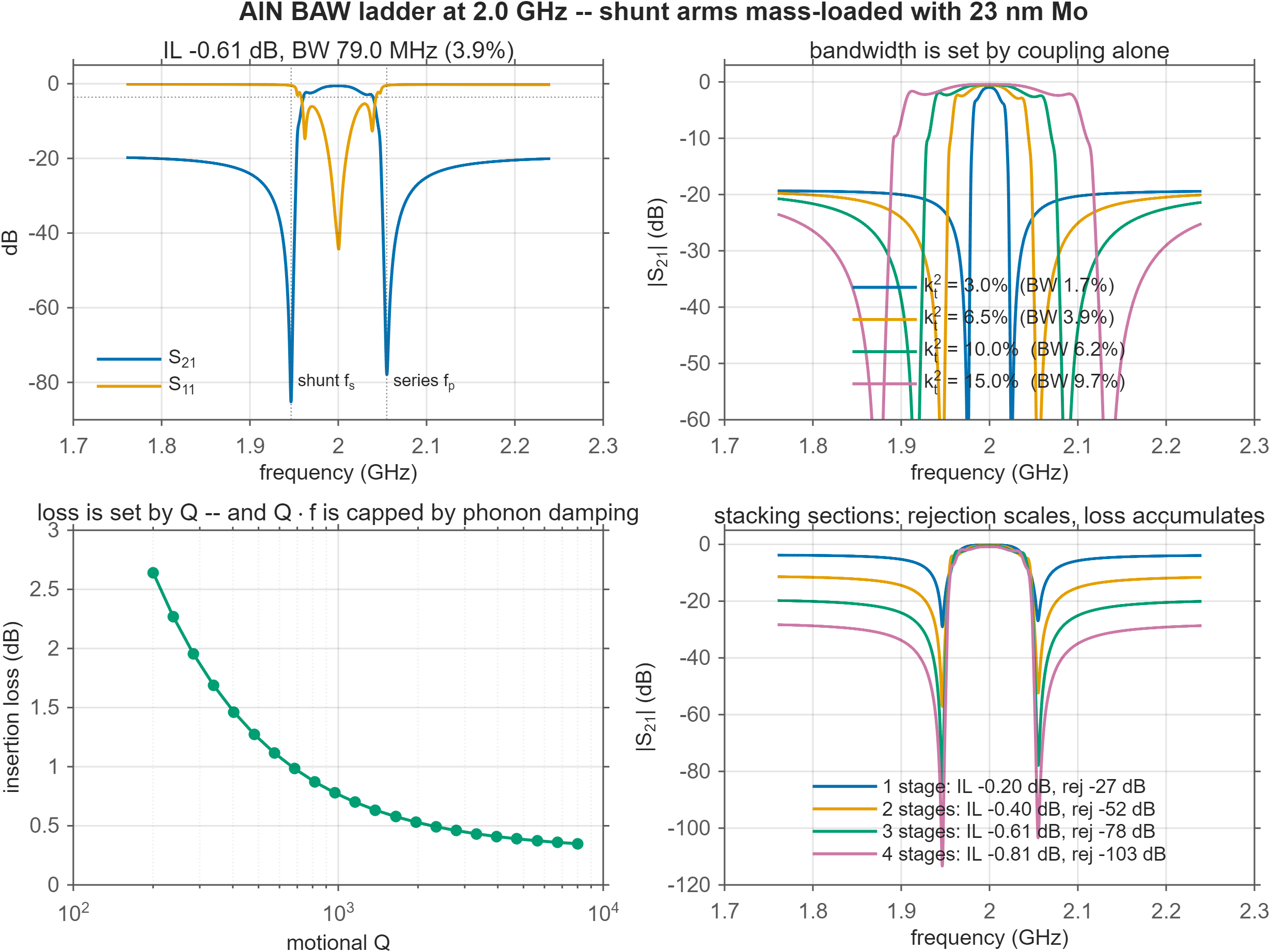
Physical parameters → mBVD circuit → impedance and S-parameters → Q and kt² extracted from the swept response the way a VNA would. Sauerbrey mass sensitivity, detection limit, and a three-stage ladder filter whose mass-loading layer is computed in nanometres of molybdenum.
modules/radar
Phased Array · Signal Processing
A real 77 GHz FMCW chain: waveform → transmitter → two-way free space → RCS target on a moving platform → receiver → dechirp → range-Doppler. Plus an analytic Monte Carlo against the bound, showing the threshold cliff.
modules/lidar
Statistics & ML
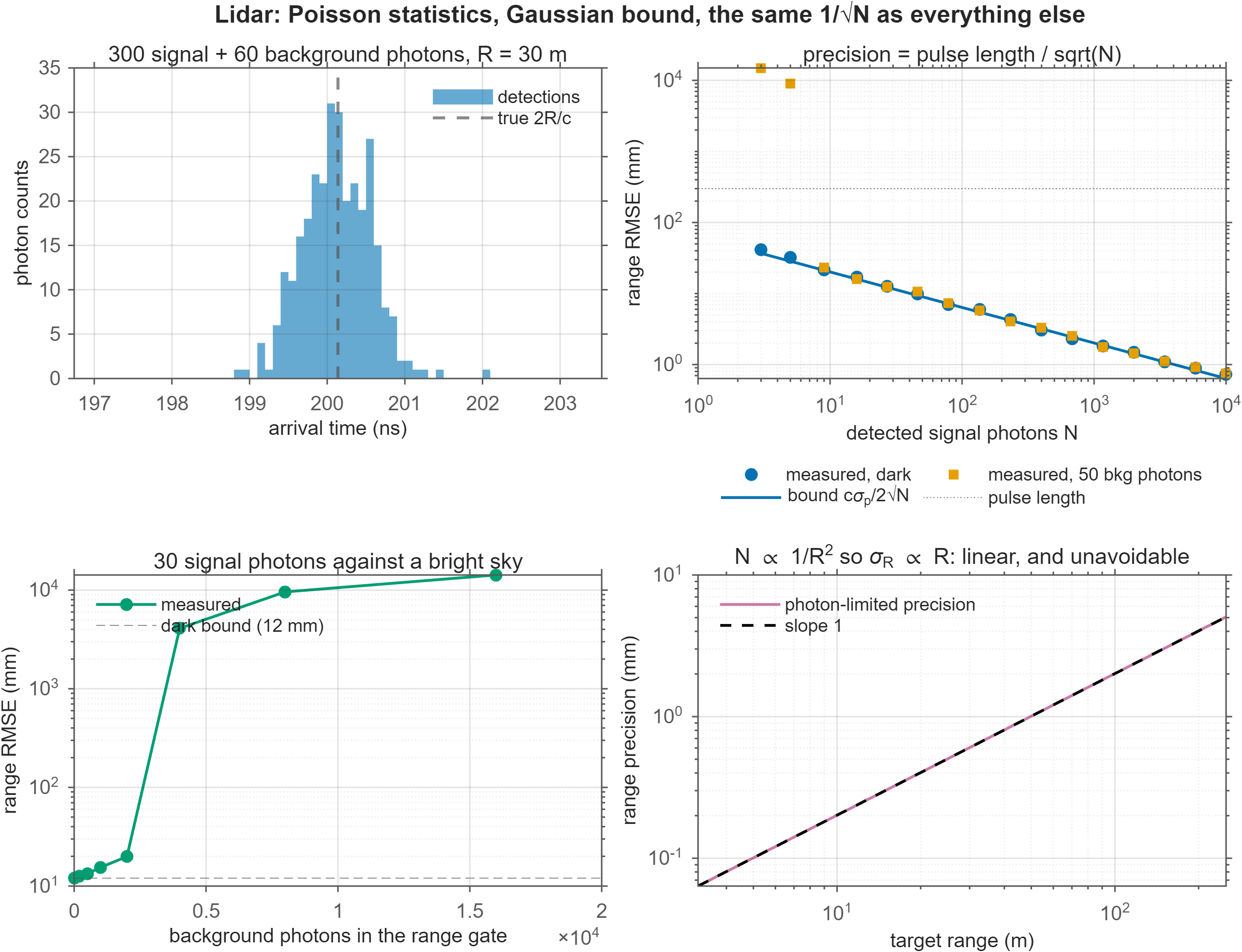
Photon-counting time of flight. A 1 ns pulse is 30 cm of light; with 10,000 photons the precision is 3 mm. Then background light, and the 1/R² photon budget that makes σR grow linearly with range.
modules/quantum
Symbolic Math
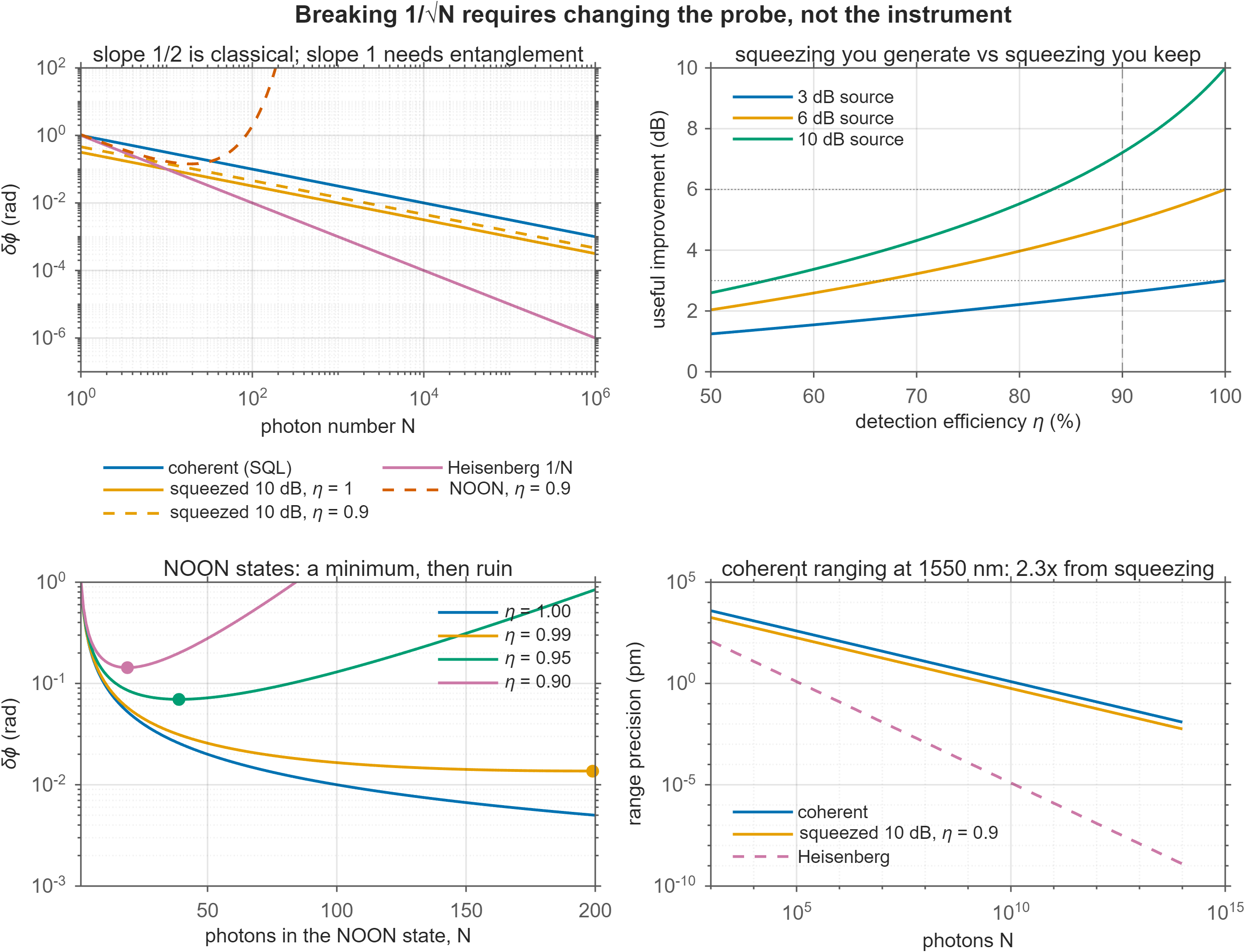
Quantum Fisher information for coherent, squeezed and NOON probes, with detection loss. Two results are derived symbolically, not asserted: that Poisson statistics give Var(n) = ⟨n⟩ and hence 1/√N, and that a lossy NOON state is optimal at exactly N = −2/ln η photons.
modules/unified
—
The capstone figure. Fits the log-log exponent of every modality and measures how far each real instrument sits from its own bound.
simulink/
Simulink · Control System
The readout system, not the device. A phase-locked loop tracks the resonance while flicker noise pushes it around and an analyte binds at t = 2 s. Built by script, so it is reviewable in a diff.
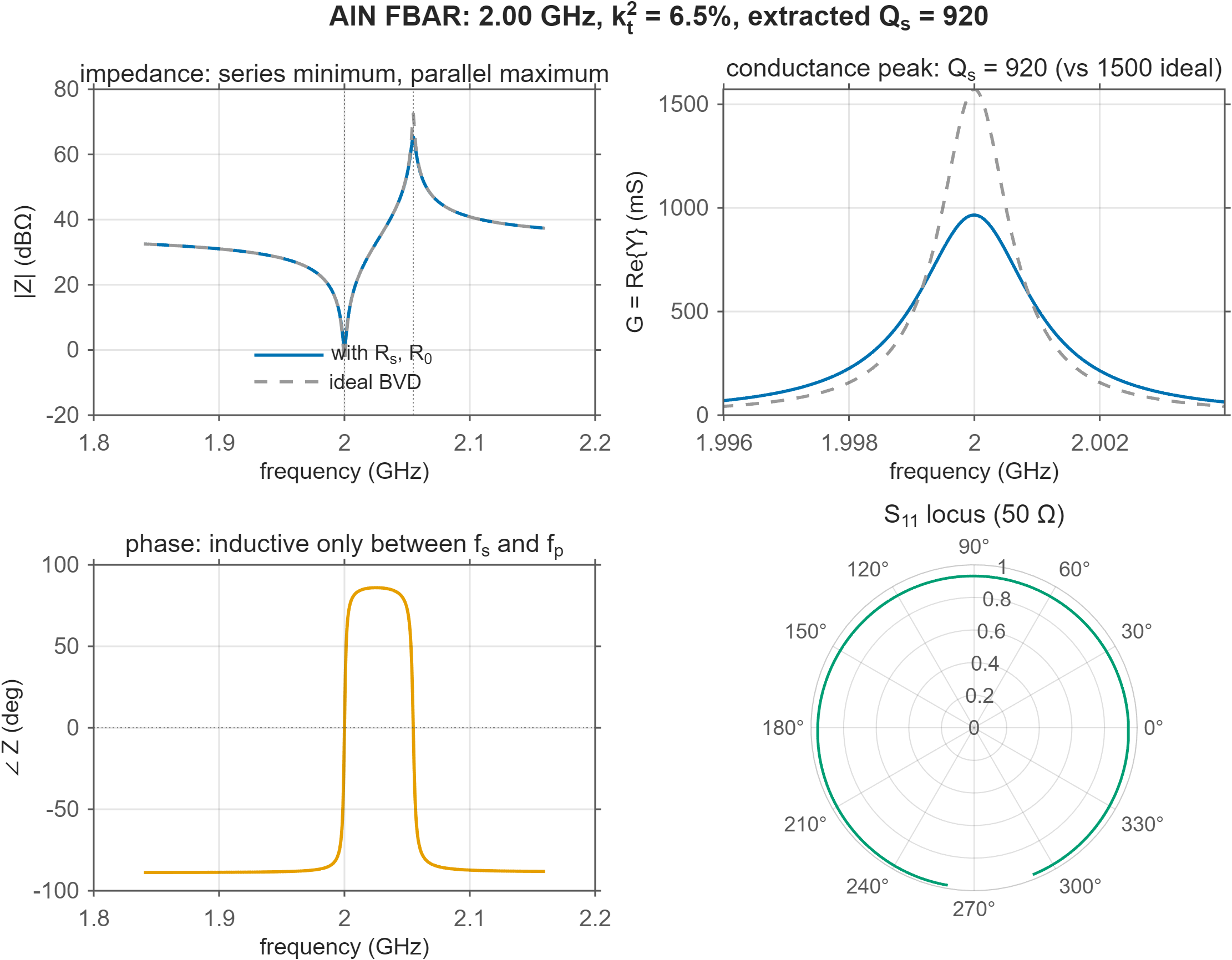
mBVD to measured Q. Electrode resistance eats 38.6% of the motional Q — the first thing that kills a real device.
0.61 dB insertion loss, 3.95% bandwidth, 85 dB rejection. The shunt arms are detuned by 23 nm of Mo — computed from the same Sauerbrey equation the biosensor uses.
Resolution is 15 cm; precision at 20 dB is 0.21 mm. A factor of 700, and the two are routinely conflated in datasheets.
Precision is pulse length divided by √N. And since N ∝ 1/R², range precision degrades linearly with distance for reasons nothing to do with the electronics.
10 dB of squeezing at 90% efficiency delivers 7.2 dB. A lossy NOON state is optimal at nineteen photons and worse for every one after. That is why squeezed light is in gravitational-wave detectors and NOON states are in papers.
Verification
Tests that assert physics, not code paths
Twenty-six of them. Each asserts a claim made in prose somewhere in this project, so that if the prose stops being true the build goes red.
the IEEE Std 176 tangent form under-reads and the linearised form over-reads — they bracket the truth, so quoting one alone is a one-sided error bar
extractedQMatchesInput…
Q recovered from the conductance half-power bandwidth equals the Q that went in, to 0.5%
sauerbreyReproducesTheTextbookQCM
the 5 MHz AT-cut constant comes out at 0.0566 Hz per ng/cm²
lodIsFlatInFrequencyAtConstantQf
sensitivity scales as f², LOD does not move — to 1e−9
ladderCascadeAgreesWithNodal…
the ABCD cascade matches a hand-solved voltage divider to 1e−10 — two independent derivations, one answer
reflectionAgreesWithRFToolbox
S11 matches RF Toolbox z2s to 1e−10
massLoadingThicknessIsPlausible
the shunt detune lands at 23 nm of Mo — a units error would surface here immediately
radarEstimatorReachesItsBound
Monte Carlo efficiency stays in [0.65, 1.5] above threshold
lidarObeysInverseRootN
fitted exponent = −0.5 ± 0.05
lossyNoonOptimumMatchesClosedForm
the numerical minimum sits at −2/ln η, ±1 photon
Reproducing it
Clone and run
>> run_all % every figure, then the test suite (~90 s)>> run_all('Tests', false) % figures only>> run_all('Only', [3 7]) % just the two headline figures>> runtests('tests/tOntos.m') % verification on its own (~2 s)% or use the library directly
p = fbarParams('f_s', 2.4e9, 'kt2', 0.15, 'Q', 900); % a ScAlN device
m = fbarResonances(p); % f_s, f_p, Q, k_t^2 from the sweep
L = fbarLOD(p, 'Pc_dBm', -20); % detection limit + Allan bathtub
F = fbarLadder(p, 'Stages', 4); % four-stage ladder and its S-parameters
Product
Needed for
MATLAB R2025b
everything
Simulink
the readout loop
Control System
flicker-noise shaping filter
Signal Processing
windowing in the radar demo
Statistics & ML
Poisson photon arrivals
Symbolic Math
the two derivations in the quantum module
RF Toolbox
the independent S-parameter cross-check
Phased Array
the FMCW radar chain
The FBAR module — the core of the repository — needs base MATLAB only. That is deliberate: the physics should not be behind a licence.
Honest accounting
What this is not
Stated plainly, because a showcase that oversells itself is worth less than one that doesn't.
The mBVD model is lumped and one-dimensional. No spurious lateral modes, no thickness-field non-uniformity, no acoustic leakage into the substrate, no temperature coefficient. Real FBARs have all four, and they are usually what limits the device. A Mason or KLM stack model, or a piezoelectric FEM, is the next step up.
The Sauerbrey relation assumes a rigid, thin, non-slipping layer. In liquid, or with a viscoelastic film, it over-reads and you need Kanazawa–Gordon or a full viscoelastic treatment. High-frequency devices are worse off here, not better, because the acoustic decay length in liquid falls as 1/√f. Any FBAR biosensor LOD quoted from Sauerbrey alone, in liquid, has not been earned.
The material values are order-of-magnitude figures assembled to support a scaling argument, not a materials database. Q·f varies by a factor of several between a research coupon and a production part.
The quantum module computes bounds, not experiments. No optical loss budget, no laser phase noise, no atmospheric turbulence. Real coherent lidar sits many tens of dB above these numbers, for the same species of reason the FBAR sits 43 dB above its own floor.
No measured data. Everything is simulation and closed-form theory. Where a number matches the literature — AlN at 35.9 MRayl, the 5 MHz QCM constant, 23 nm of Mo, a 0.6 dB / 4% BAW filter — that is a consistency check, not a validation.